


Arithmetization in zk-STARKs

In our last piece, we took a deep dive into polynomial commitment schemes, taking a closer look at the renowned KZG10 scheme. Despite many benefits of KZG10, it has a notable shortcoming - the need for a trusted setup. Addressing this issue, we will shift our focus to transparent proofs, also known as zk-STARKs, which eliminate the need for any trusted party.
STARKs
zk-STARKs (Zero-Knowledge Scalable Transparent ARguments of Knowledge) are a type of cryptographic proof system that allows one party (the prover) to demonstrate to another party (the verifier) that a specific statement is true, without revealing any information about the underlying data or the statement itself. zk-STARKs are a subset of zero-knowledge proofs and offer several key characteristics that make them attractive:
Zero-knowledge: zk-STARKs enable provers to show the validity of a statement without revealing any information about the statement or the data it is based on, ensuring privacy in sensitive applications.
Scalability: zk-STARKs are designed to handle complex statements and large datasets efficiently, making them suitable for applications that require high-performance cryptographic proofs.
Transparency: Unlike SNARKs, zk-STARKs do not require a trusted setup. This makes them more secure and easier to deploy in decentralized systems like blockchains, where trust assumptions can be problematic.
Post-quantum security: zk-STARKs are believed to be resistant to attacks from quantum computers due to their reliance on different cryptographic assumptions.
STARKs leverage hash-based commitments, subsequently employing the FRI-protocol to prove the low-degree nature of a polynomial. The acronym FRI stands for Fast Reed-Solomon Interactive Oracle Proof. The protocol was introduced by Eli Ben-Sasson and others in their 2016 publication, "Fast Reed-Solomon Interactive Oracle Proofs of Proximity." Building upon this, the comprehensive zero-knowledge protocol was outlined in the 2018 STARK paper by the same team. This work laid the foundation for the establishment of Starkware, co-founded by Ben-Sasson.
With this knowledge of STARKs, let's delve deeper into the intricacies of their work.

Statement
Starting off, it's essential to identify the problem we are working with. In the realm of zero-knowledge proofs, we refer to this as a "statement." This term is also used in the zk-STARK paper. Throughout this article, we will follow the STARK terminology, which might occasionally deviate from what's used in other SNARKs.
In our case, we are going to prove that we know the 12th number in the Lucas sequence (we don’t want to bore people with another example based on the Fibonacci sequence).

Wondering what Lucas numbers are? The Lucas sequence begins with 2 followed by 1. After that, every number in the sequence is the sum of its two immediate predecessors. Here's how the sequence shapes up: 2, 1, 3, 4, 7, 11, 18, 29... and so on. If it reminds you of another well-known sequence, it's purely coincidental!
Computers are not fans of calculating massive numbers, so let's work within a finite field of 97. If the terms 'finite fields' and 'modular arithmetic' sound a bit rusty, take a look at our previous article linked here. In essence, when we talk about operating in a finite field, it means that the integers we work with don't go on forever. Instead, they hit a limit (or a "modulus") and then loop back to the beginning. Think of how clocks work within a finite field of 12 hours, or how a day goes in a finite field of 24 hours.
Now, while determining the 12th Lucas number doesn't inherently pose challenges, we're using the finite field of 97 for illustrative purposes. So, when working within this field, the Lucas sequence looks like this: 2, 1, 3, 4, 7, 11, 18, 29, 47, 76, 26… and so on. No number in this sequence will ever surpass 97.
In the context of our STARK, we will skip the initial four numbers, targeting the twelfth element as our final entry. This forms the basis of our statement. To phrase this more formally, given the modulo 97:
The prover knows it. The verifier doesn’t and doesn't want to spend time computing it.
Arithmetization
Arithmetization in STARKs is split between the following steps: (1) creation of the execution trace, (2) interpolation of the polynomial, (3) extending the domain of the polynomial
Step (1): Building the trace requires connecting each step of the computation with an element of a finite field in a structured way, such that it can be succinctly represented as an evaluation of a polynomial. This will allow the prover to commit to a single polynomial instead of committing to all elements in the execution trace individually.
Our computation is the computation of the 12th Lucas number. Each step of the computation is a Lucas number from the 5th to the 12th. These are the elements of our trace.
The trace is usually a matrix where each row corresponds to a different step in the computation, and each column corresponds to a different state variable. In our case, the computation is simple enough that there is only one state variable: the current Lucas number. This means our trace will be a single column.

The trace will be a representation of a polynomial p evaluated at values in the trace. As such, the results of the evaluation will be related to the trace.
The next step is to create a multiplicative group of order 96 (since the first element is 0) within our field = 97. A multiplicative group is a subset of a field where the operation is multiplication, excluding the zero element. This group is cyclic, which means there exists a generator g such that all other elements in the group can be written as powers of g. Each element of the trace should be associated with a different element of a multiplicative subgroup of the finite field.
We want to find an 8-element subgroup, and we need a generator 𝑔 in 𝔽 whose multiplicative order is 5. The elements of group G will serve as a coordinate x for our polynomial p.
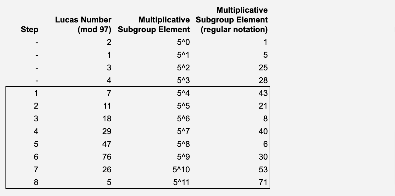
The process of finding a generator for a finite field is trial and error. We start by picking an arbitrary element g from the field, then compute the powers of g modulo p until we reach
If we encounter 1 before reaching
then g is not a generator, and we should try a different element. If we reach it without encountering 1, then g is a generator of the field.
We can automate this process by using a simple Python program:
def find_generator(p):
    for g in range(2, p):
        powers = set()
        for i in range(1, p):
            powers.add(pow(g, i, p))
        if len(powers) == p-1:
            return g
    return -1

print(find_generator(97))
This process might take a while for large primes, but it should be quick for p = 97.
Step (2): Next, we aim to find a polynomial p(x) with a degree less than 8. This polynomial, when provided with the respective element of the multiplicative subgroup as input, will compute the Lucas number at each computational step. In essence:
where L represents the Lucas number.
For each element of g, the polynomial will take values such that
Now, let's interpolate this polynomial. We have a couple of methods to choose from: one is the Lagrange interpolation (discussed in the prior article) and the other is the Number Theoretic Transform (NTT). The NTT is similar to the Fast Fourier Transform (FFT) but functions within finite fields. For a more in-depth understanding of NTT, you might want to check out Vitalik's article on the subject.
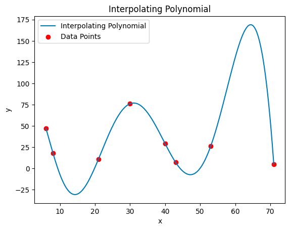
Our polynomial p, has a degree 7, given that our trace comprises 8 elements. This polynomial, rounded to full integers, can be represented in coefficient form as:
When we plot this polynomial on the coordinate plane, it looks as presented below. Keep in mind that what we are visualizing is the standard depiction of the polynomial. This visualization helps in making it more intuitive to understand the concept of low-degree extension we will undertake in the subsequent step.
For interested, below is a Python code that performs the Lagrange interpolation:
import galois
import numpy as np
# Create the finite field
GF = galois.GF(97)
# Define your generator
g = GF(5)
# Define the x and y values as galois.Array
x_values = GF([g**i for i in range(4, 20)]) # Convert list to GF(97) array
y_values = GF([7, 11, 18, 29, 47, 76, 26, 5, 31, 36, 67, 6, 73, 79, 55, 37]) # Convert list to GF(97) array
# Compute the Lagrange interpolating polynomial
L = galois.lagrange_poly(x_values, y_values)
# Print the polynomial
print("Lagrange Polynomial:", L)
# Verify that the polynomial evaluates correctly at the given points
assert np.array_equal(L(x_values), y_values), "The polynomial does not interpolate the points correctly."
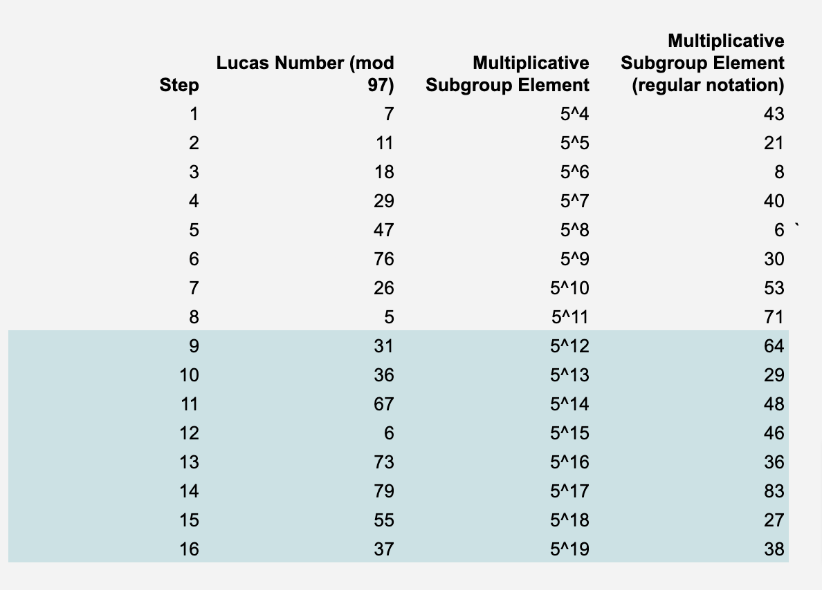
print("Verification passed: Polynomial matches the provided points.")Step (3): Our next move is to extend the polynomial's domain. Within the STARKs framework, this equals evaluating the polynomial at extra points. For our purposes, we will double the domain, so there's redundancy to reconstruct the polynomial even if some original data points go missing. Typically, these extensions are much larger.
It's important to keep the new set of trace elements as a power of 2. This is required for the NTT, though it's not essential for Lagrange interpolation. When dealing with truly large polynomials (like those in practical applications), the interpolation is primarily executed using NTT, which has log-linear computational complexity (you read more about computational complexity types in this article - it is a must-read for zk enthusiasts). Given that interpolating the polynomial is arguably the most resource-intensive part of the entire protocol, any efficiency gains, like those offered by the NTT, are invaluable.
For our purposes, selecting random points on the polynomial will suffice. However, in real-world scenarios, an additional shift in the polynomial is calculated within the field. This step helps hide the original data, enhancing privacy. Now, let's visualize our polynomial within the expanded domain. Keep in mind, that this is a depiction of the polynomial on a Euclidean plane and not in a finite field.

Degree extension provides the redundancy to reconstruct the original polynomial if some data from the initial eight points goes missing. The Unisolvence Theorem tells us that a polynomial p(x) of degree n is uniquely defined when its values are at n + 1 distinct points.
If you're given n + 1 unique points, there is only one polynomial p(x) with a degree up to n that satisfies the expression:
This essentially means that for n+1 unique points, there's a single polynomial, with a degree no greater than n, that intersects all these points. This polynomial is referred to as the interpolating polynomial. Thus, with n+1 points on this polynomial, we can retrieve any polynomial of degree n.
Within STARKs, this kind of polynomial serves two primary functions. First, the FRI protocol verifies its low-degree. In our scenario, the polynomial's degree of less than 8 is low. Secondly, this polynomial acts as a foundational component for Reed-Solomon codes, which encode data blocks as polynomials over a finite field. When transmitting data, errors may occur, and some values may be received incorrectly. The task is then to recover the original polynomial, even if some values are erroneous.
This recovery is possible due to the properties of polynomials and the fact that more evaluations of the polynomial are sent than the minimum required by the Unisolvence Theorem. By evaluating the polynomial at more points, we can tolerate some errors and still uniquely recover the original polynomial, even if some of the received values are incorrect. This is what allows Reed-Solomon codes to correct errors in data transmission.

Returning to our data: we have encoded a polynomial based on the following trace. We expanded the domain of our initial polynomial by selecting extra random points that the polynomial passes through. Now it’s time to commit to this data.
The commitment process involves hashing the values representing our polynomial and constructing a Merkle tree using these hashes. Every data point, along with its subsequent branches, must be hashed. The root of the hash is then sent to the verifier. Let's take a look at its visual representation of a Merkle tree.

Here we come across the Fiat-Shamir. The Fiat-Shamir heuristic is a method used to convert an interactive proof, into a non-interactive proof.
The Fiat-Shamir heuristic turns this interactive proof into a non-interactive one by replacing the verifier's role with a cryptographic hash function. Instead of the verifier asking random questions, the prover computes the hash of the statement and previous responses to generate the next challenge. Depending on the specifics of the protocol, this might involve interpreting the hash as an integer and perhaps reducing it modulo some value. The exact way the hash is turned into a challenge depends on the details of the particular protocol being used. This allows the prover to create a proof without interacting with the verifier.
The heuristic's security is based on the assumption that the hash function behaves like a random oracle, meaning that it's computationally infeasible to predict its output without actually computing it.
Constraints
Let's revisit the constraints we outlined at the start of our discussion, but this time we will adjust them to align with the expanded domain.
Basic Constraints:
Given the Lucas sequence, if we begin with the fifth number, add the sixth, and keep summing the last two numbers for six consecutive iterations, the sixteenth number, when reduced modulo 97, is 37. In formal terms:
The first element,
a[0] = 7The second element,
a[1] = 11The Lucas sequence rule,
an = an−1 + an−2,is valid for elements2 < n <= 14The final element
a[15] = 37
Polynomial Constraints:
Earlier, we transformed the execution trace that describes the problem into polynomial p. Now, we will rewrite the constraints into polynomial form based on the trace polynomial p. The trace and its corresponding values are denoted with a and ai. When presented as constraints in polynomial terms, it will look like this:
When we evaluate the polynomial p at the specific trace value gi, it yields the corresponding number from the Lucas sequence. This happens because we have mapped the elements of the group G with the numbers from the Lucas sequence and interpolated the polynomial based on this mapping.
Now, the third constraint, which is more challenging:
Putting it more simply: when we evaluate the polynomial p at the ith element of x, the outcome is
This holds true for i values from 6 to 18, but no further, since these are the last two elements of the trace. The last element is described by the fourth constraint, while the one before cannot be calculated by the formula.
We have now translated our constraints into a polynomial form, echoing the exact constraints we started with. Hence, if these polynomial constraints hold up, then our initial statement is true.
Root Constraints
We will now transition from the polynomial form to the root form. When discussing polynomials, a root is essentially a value, let's say x = a, where the polynomial p(x) evaluates to zero. In simpler terms, if p(a) = 0, then a is considered a root of the polynomial p(x). Let's see how our constraints look like in the root format:
By this logic, if the values of x are the roots of p(x), then our initial statement is true.
Rational Functions Constraints
Based on the Polynomial Remainder Theorem when we divide a polynomial p(x) by x − z, the remainder is p(z). So, if p(z) = 0, it means that the division by x − z yields no remainder. This indicates that x − z is a factor of p(x), and consequently, z is a root of the polynomial p(x). As a result, there must exist another polynomial, say t(x), such that when t(x) is multiplied by x − z, we get p(x).
Example:
Given
if we think x − 2 might be a factor, we can test it by calculating P(2) = 4 − 10 + 6 = 0. We confirm that indeed P(2) = 0, so x−2 is a factor. Now, when we divide p(x) by x − 2 the quotient is x − 3 and there is no remainder. So:
Now, let’s transform the root constraints into rational functions.
Before moving forward let's dive deeper into the third constraint. Calculating the product of all the elements of g might seem daunting, especially when we aim for efficiency. Fortunately, there's a neat workaround that can make that job much easier.
Instead of the heavy calculation in the denominator, we can simply use:
The key point: in group G, raising g to the power of N gives us 1. It can be easily verified that:
Given this observation, if we factor the polynomial x^N-1 over the field, the roots are precisely the powers of g. Therefore x^N-1 can be expressed as a product of linear terms:
This is an illustration of the fundamental theorem of algebra which says that a polynomial of degree N has exactly N roots in a field containing those roots. In this context, the field contains the cyclic group generated by g, and x^N−1 has its roots as the powers of g.
The equation holds because every power of g is a root of x^N−1, and the polynomial can be expressed as a product of linear terms based on these roots.
In our case, since the trace has only 16 steps, the calculation will be manageable, so we will keep the constraint as is. To apply the simplification for our F = 97 and with only 16 trace steps, we would have to cancel all the remaining 81 steps/polynomials, which would cost us dearly in terms the cost of compute.
We have now transformed the constraints from the root form to the rational function form. Since in each case the division leaves no remainder, the results are always polynomial.
We now can re-write the constraints as polynomials:
If these statements are polynomials, then our initial statement holds.
After transitioning our constraints from the basic form to rational functions, our next and final step is to create the composition polynomial denoted c(x).
The composition polynomial is created by multiplying our rational functions with a random value, α, from the field and then adding the results:
If f statements are polynomials, then c(x) is guaranteed to be a polynomial too. The next step is to use a Merkle Tree to commit to c(x).
And this commitment finalizes the zk-STARK's arithmetization. Though less intuitive than the SNARKs' arithmetic circuit method, the trace technique scales better and is apt for sequential and repetitive computations.
Summary
Let's take a step back and recap the steps and tools we used:
Problem Statement: Our goal was to prove the knowledge of the twelfth number in the Lucas sequence.
Algebraic Execution Trace: We constructed the algebraic execution trace, detailing the computation step by step. We limited the calculation to a field of 97 elements generated by a single element g.
Transformation to Polynomials: We converted the trace to a polynomial using Lagrange Interpolation. For larger traces Fast Fourier Transform over finite fields (aka Number Theoretic Transform) would be a more efficient choice.
Domain Extension: We extended the polynomial through the addition of more points that lay on this polynomial. This ensures we can reconstruct the polynomial even if some of the original points are lost. The data recovery method with use of polynomials is called Reed-Solomon codes.
Polynomial Commitment: We committed to the polynomial by hashing it into a Merkle Tree, which is then send by a prover to verifier. With the help of Fiat-Shamir heuristic that introduces randomization based on the resulting hashes, we can make the protocol non-interactive.
Constraints Transformation: We described the constrains and transformed them subsequently to polynomial, root and then rational function form. From these functions we then formed the composition polynomial. Successfully proving that the composition polynomial is low-degree is equal to confirming that the original statement is true.
Indeed, in the next article, we will show how the FRI protocol is used to prove that the composition polynomial is low-degree. Keep an eye out for that!
P.S. I'm aiming to release the next piece sooner than in 6 months. Thanks for your patience.
I couldn’t write this blogpost without the following sources:
Starkware, STARK101, (main inspiration and source)
Starkware, Arithmetization
Starkware, ethSTARK
Aleksander Berentsen, Jeremias Lenzi, Remo Nyffenegger, A Walkthrough of a Simple zk-STARK Proof
RISC Zero, STARK by hand